13 `geopandas`

GeoPandas is a Python library that extends the pandas library by adding support for geospatial data. In this lesson we will introduce the geopandas library to work with vector data. We will also make our first map.

To begin with, let’s import geopandas with its standard abbreviation gpd:

# this is the library we will explore
import geopandas as gpd

# we will start using matplotlib for making maps
import matplotlib.pyplot as plt

13.1 Data

In this lesson we will use simplified point data about wild pigs (Sus scrofa) sightings in California, USA from the Global Biodiversity Information Facility.

We can read in a shapefile with geopandas by using the gpd.read_file() function.

pigs = gpd.read_file('data/gbif_sus_scroga_california/gbif_sus_scroga_california.shp')
pigs.head()

	gbifID	species	state	individual	day	month	year	inst	collection	catalogNum	identified	geometry
0	899953814	Sus scrofa	California	NaN	22.0	3.0	2014.0	iNaturalist	Observations	581956	edwardrooks	POINT (-121.53812 37.08846)
1	899951348	Sus scrofa	California	NaN	9.0	6.0	2007.0	iNaturalist	Observations	576047	Bruce Freeman	POINT (-120.54942 35.47354)
2	896560733	Sus scrofa	California	NaN	20.0	12.0	1937.0	MVZ	Hild	MVZ:Hild:195	Museum of Vertebrate Zoology, University of Ca...	POINT (-122.27063 37.87610)
3	896559958	Sus scrofa	California	NaN	1.0	4.0	1969.0	MVZ	Hild	MVZ:Hild:1213	Museum of Vertebrate Zoology, University of Ca...	POINT (-121.82297 38.44543)
4	896559722	Sus scrofa	California	NaN	1.0	1.0	1961.0	MVZ	Hild	MVZ:Hild:1004	Museum of Vertebrate Zoology, University of Ca...	POINT (-121.74559 38.54882)

One shapefile = multiple files

Although the parameter for gpd.read_file() is only the .shp file, remember that we need to have at least the .shx and .dbf files in the same directory as the .shp to read in the data.

13.2 `GeoSeries` and `GeoDataFrame`

The core data structure in GeoPandas is the geopandas.GeoDataFrame. We can think of it as a pandas.DataFrame with a dedicated geometry column that can perform spatial operations.

The geometry column in a gpd.GeoDataFrame holds the geometry (point, polygon, etc) of each spatial feature. Columns in the gpd.GeoDataFrame with attributes about the features are pandas.Series like in a regular pd.DataFrame.

Example

First of all, notice that the leftmost column of pigs is a column named geometry whose values indicate points.

pigs.head(3)

	gbifID	species	state	individual	day	month	year	inst	collection	catalogNum	identified	geometry
0	899953814	Sus scrofa	California	NaN	22.0	3.0	2014.0	iNaturalist	Observations	581956	edwardrooks	POINT (-121.53812 37.08846)
1	899951348	Sus scrofa	California	NaN	9.0	6.0	2007.0	iNaturalist	Observations	576047	Bruce Freeman	POINT (-120.54942 35.47354)
2	896560733	Sus scrofa	California	NaN	20.0	12.0	1937.0	MVZ	Hild	MVZ:Hild:195	Museum of Vertebrate Zoology, University of Ca...	POINT (-122.27063 37.87610)

As usual, we can check the type of our objects using the type Python function:

# type of the pigs dataframe 
print(type(pigs))

# type of the geometry column
print(type(pigs.geometry))

# type of the gbifID column
print(type(pigs.gbifID))

<class 'geopandas.geodataframe.GeoDataFrame'>
<class 'geopandas.geoseries.GeoSeries'>
<class 'pandas.core.series.Series'>

The new data type of the geometry column is also reflected when we look at the data types of the columns in the data frame:

pigs.dtypes

gbifID           int64
species         object
state           object
individual     float64
day            float64
month          float64
year           float64
inst            object
collection      object
catalogNum      object
identified      object
geometry      geometry
dtype: object

We can also check the type of each element in the geometry column using the geom_type attribute of a gpd.GeoDataFrame:

pigs.geom_type

0       Point
1       Point
2       Point
3       Point
4       Point
        ...  
1041    Point
1042    Point
1043    Point
1044    Point
1045    Point
Length: 1046, dtype: object

13.3 Geometric information

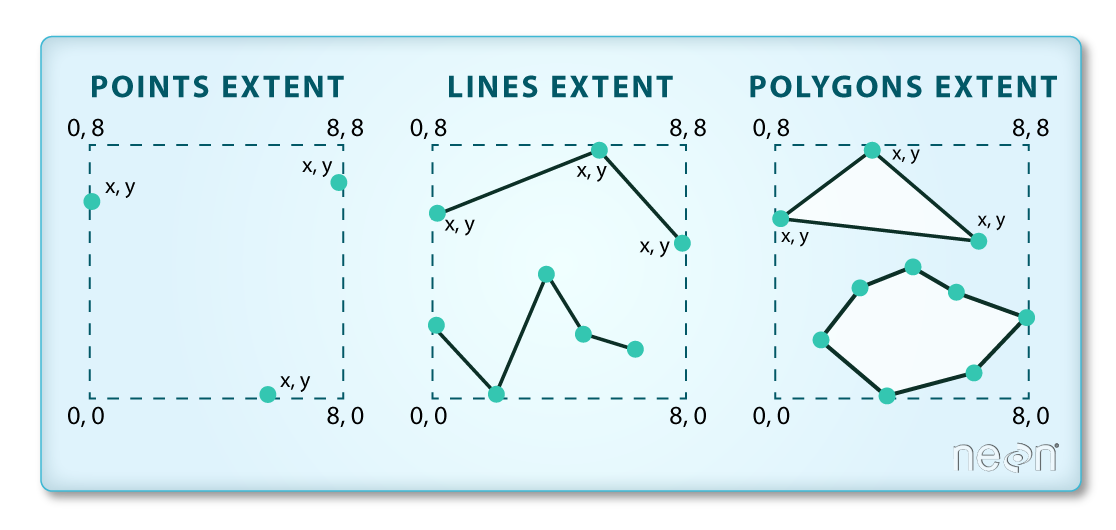
Two other important attributes of a gpd.GeoDataFrame are its coordinate reference system (CRS) and its extent.

We can think of the coordinate reference system (CRS) as the instructions to locate each feature in our dataframe on the surface of the Earth. We access the CRS of a gpd.GeoDataFrame using the crs attribute:

# access the CRS of the GeoDataFrame
pigs.crs

<Geographic 2D CRS: EPSG:4326>
Name: WGS 84
Axis Info [ellipsoidal]:
- Lat[north]: Geodetic latitude (degree)
- Lon[east]: Geodetic longitude (degree)
Area of Use:
- name: World.
- bounds: (-180.0, -90.0, 180.0, 90.0)
Datum: World Geodetic System 1984 ensemble
- Ellipsoid: WGS 84
- Prime Meridian: Greenwich

The extent of the geo-dataframe is the bounding box covering all the features in our geo-dataframe. This is formed by finding the points that are furthest west, east, south and north.

Spatial extent of different vector data. Image Source: National Ecological Observatory Network (NEON)

We access the extent of a gpd.GeoDataFrame using the total_bounds attribute:

pigs.total_bounds

array([-124.29448 ,   32.593433, -115.4356  ,   40.934296])

13.4 Data wrangling

GeoPandas is conveniently built on top of pandas, so we may use everything we have learned about data selection, wrangling, and modification for a pd.DataFrame.

Example

Suppose we only want to use recent data for wild pig observations. A quick check shows that this dataframe has data since 1818:

# use sort_index() method to order the index
pigs.year.value_counts().sort_index()

1818.0     31
1910.0      1
1925.0      1
1927.0      4
1929.0      3
         ... 
2019.0    101
2020.0    159
2021.0    164
2022.0    185
2023.0     98
Name: year, Length: 61, dtype: int64

We can use our usual data selection to get data from 2020 onwards:

# selet data from 2020 onwards
pigs_recent = pigs[pigs.year>=2020]

# print length of original dataframe
print(len(pigs))

# check length of new dataframe
len(pigs_recent)

13.5 Plotting

13.5.1 `plot()`

Similarly to a pd.DataFrame, a gpd.GeoDataFrame has a plot() method that we can call directly to create a quick view of our data. The geospatial information of the gpd.GeoDataFrame will be used to create the axes of the plot.

Example

This is a quick look at our recent pigs data:

pigs_recent.plot()

<AxesSubplot:>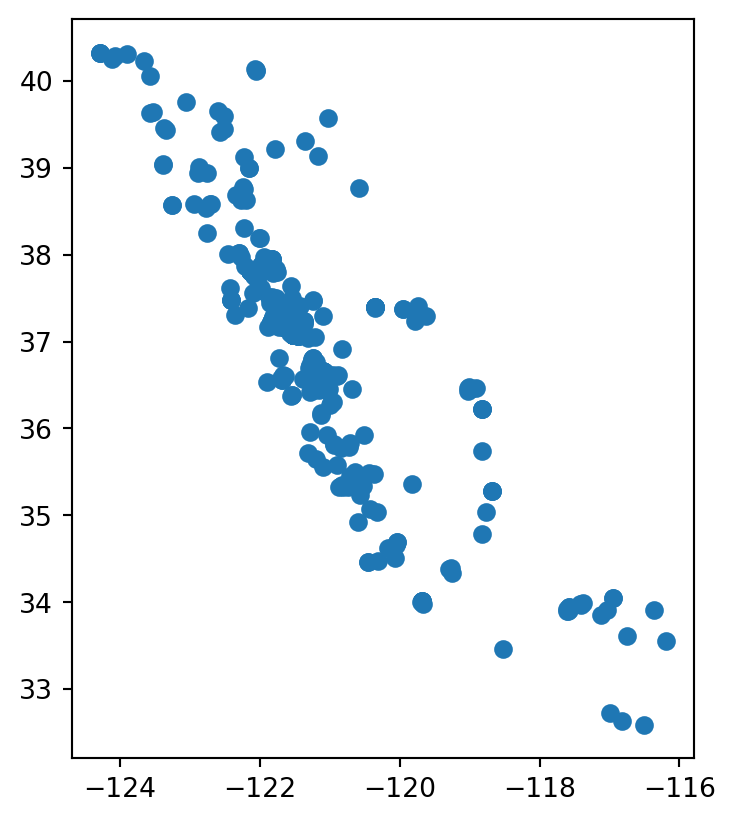

13.5.2 `matplotlib`’s `fig` and `ax`

Going forward, we will often want to make more complex visualizations where we add different layers to a graph and customize it. To do this we will use the matplotlib Python library for creating visualizations. We can interact with matplotlib via its pyplot interface, which we imported at the top of the notebook as

# import matplotlib with standard abbreviation
import matplotlib.pyplot as plt

13.6 Best practices for importing packages

We always import libraries at the top of our notebook in a single cell. If halfway through our analysis we realize we need to import a new library, we still need to go back to that first cell and import it there!

Matplotlib graphs the data in a figure which can have one or more axes. The axis is only the area specified by the x-y axis and what is plotted in it. To create a new blank figure:

Initialize a new figure and axes by calling pyplot’s subplots() function, and
show the graph using plt.show():

# create a blank figure (fig) with an empty axis (ax)
fig, ax = plt.subplots()

# display figure
plt.show()

Notice we get a figure with a single empty axis. We can think of this step as setting a new blank canvas on which we will paint upon.

Functions with multiple return values

Notice that plt.subplots() is a function that returns two objects (has two outputs).

13.6.1 Adding a layer

When using matplotlib, it can be useful to think of creating a plot as adding layers to an axis. The general syntax to plot a datafram df onto an axis is:

# create new figure and axis
fig, ax = plt.subplots()

# plot df on the ax axis
df.plot(ax=ax, 
        ...)   # other arguments for plot function

# display figure
plt.show()

Example

The first layer we want to add to our axis is the pigs_recent point data. We can plot our data using matplotlib like this:

# create new figure and axis
fig, ax = plt.subplots()

# add pigs point plot to our figure's axis
pigs_recent.plot(ax=ax)

# display figure
plt.show

<function matplotlib.pyplot.show(close=None, block=None)>

13.6.2 Customization

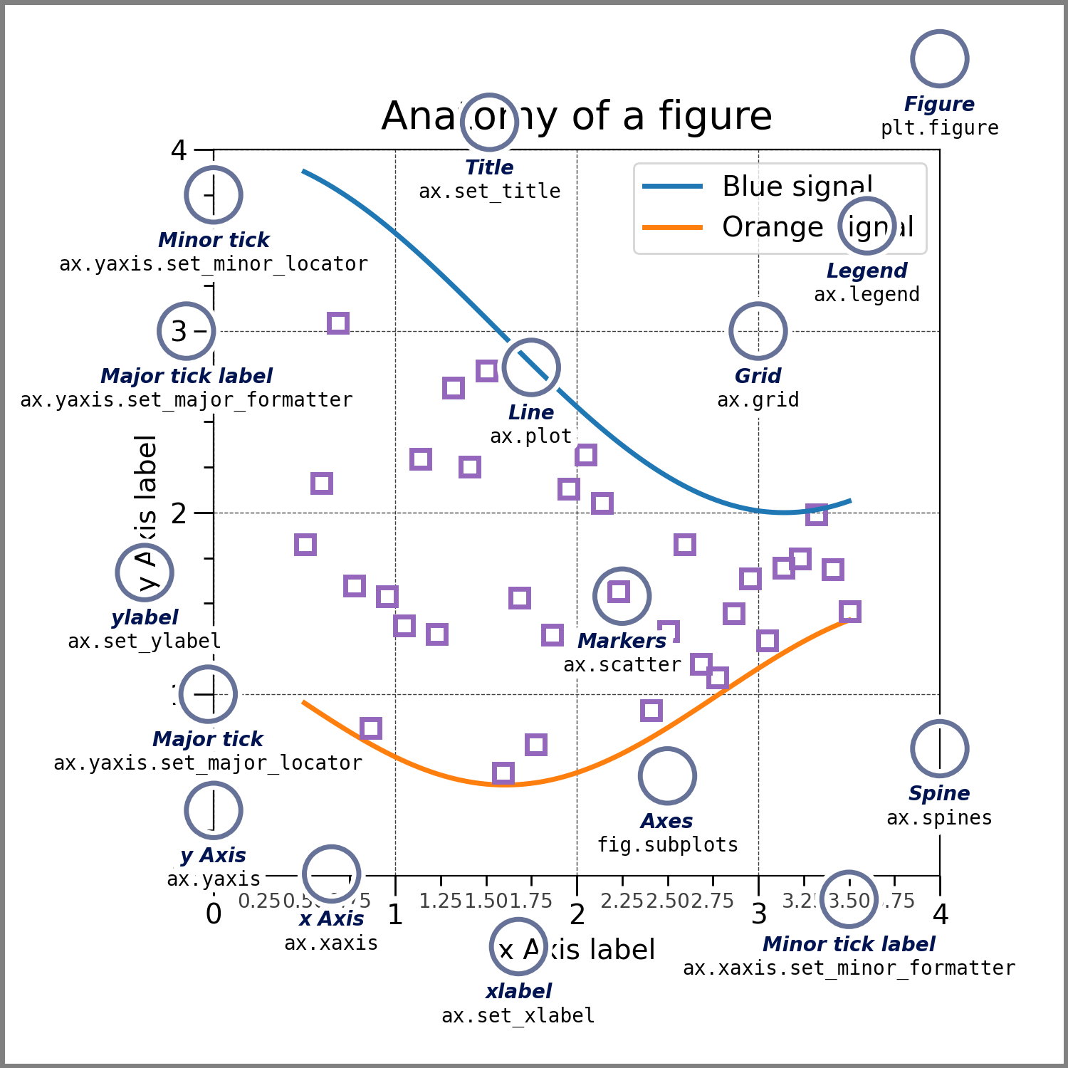
Matplotlib allows for a lot of customization. Some of it can be done directly in the plot() method for the dataframe (like we’ve done when ploting data using pandas), while other is done by updating attributes of the axis ax. The following image shows some examples of elements in the axis that can be updated.

Example

Some basic customization for our pigs data could looke like this:

# initialize empty figure
fig, ax = plt.subplots()

# add data to axis
# notice customization happens as arguments in plot()
pigs_recent.plot(ax=ax,
                 alpha=0.5,
                 color='brown'
                 )

# update axis 
# customization separate from the data plotting
ax.set_title('Reported "Sus scrofa" sightings in CA (2020-2023)')
ax.set_xlabel('Longitude')
ax.set_ylabel('Latitude')

# display figure
plt.show()

13.7 Simple map

We can add multiple layers of shapefiles to our maps by plotting multiple geo-dataframes on the same axis.

Example

We will import a shapefile with the outline of the state of CA. The original shapefile was obtained through the California’s government Open Data Portal, and the one used here was updated to match the CRS of the points (we’ll talk more about matching CRSs later).

# import CA boundary
ca_boundary = gpd.read_file('data/ca-boundary/ca-boundary.shp')
ca_boundary

	REGION	DIVISION	STATEFP	STATENS	GEOID	STUSPS	NAME	LSAD	MTFCC	FUNCSTAT	ALAND	AWATER	INTPTLAT	INTPTLON	geometry
0	4	9	06	01779778	06	CA	California	00	G4000	A	403501101370	20466718403	+37.1551773	-119.5434183	MULTIPOLYGON (((-119.63473 33.26545, -119.6363...

We can see this geo-dataframe has a single feature whose geometry is MultiPolygon. Plotting the California outline with the point data is easy: just add it as a layer in your axis.

# initialize an empty figure 
fig, ax = plt.subplots()

# add layers
# add CA boundary
ca_boundary.plot(ax = ax,
                color = 'none',
                edgecolor = '#362312')

# add pig point data
pigs_recent.plot(ax = ax,
                alpha = .5,
                color = '#FF5768',
                edgecolor = '#FFBF65')

# customization
ax.set_title('Reported "Sus scrofa" sightings in CA (2020-2023)')
ax.set_xlabel('Longitude')
ax.set_ylabel('Latitude')

# display figure
plt.show()

13.8 References

GBIG data: GBIF.org (23 October 2023) GBIF Occurrence Download https://doi.org/10.15468/dl.qavhwp

Geopandas Documentation - Introduction to GeoPandas

Matplotlib Documentation - Basic Usage

NEON tutorials - Intro to Vector Data in R

13.1 Data

13.2 GeoSeries and GeoDataFrame

13.3 Geometric information

13.4 Data wrangling

13.5 Plotting

13.5.1 plot()

13.5.2 matplotlib’s fig and ax

13.6 Best practices for importing packages

13.6.1 Adding a layer

13.6.2 Customization

13.7 Simple map

13.8 References

13.2 `GeoSeries` and `GeoDataFrame`

13.5.1 `plot()`

13.5.2 `matplotlib`’s `fig` and `ax`