import numpy as np
import geopandas as gpd
import rioxarray as rioxr
import matplotlib.pyplot as plt

from shapely.geometry import Polygon

# used to access STAC catalogs
from pystac_client import Client
# used to sign items from the MPC STAC catalog
import planetary_computer

# ----- other libraries for nice ouputs
from IPython.display import Image25 STAC specification
So far in our course we have accessed data in two ways: by downloading it directly from the data provider or by obtaining a URL from a data repository. This can be a convenient way to access targeted datasets, often usign GUIs (graphical user interfaces) for data discovery and filtering. However, relying on clicking and copy-pasting addresses and file names can make our workflows more error-prone and less reproducible. In particular, satellites around the world produce terabytes of new data daily and manually browsing through data repositories would it make hard to access this data. Moreover, we wouldn’t want to learn a new way to access data from every single big data provider. This is where STAC comes in.

The SpatioTemporal Asset Catalog (STAC) is an emerging open standard for geospatial data that aims to increase the interoperability of geospatial data, particularly satellite imagery. Many major data archives now follow the STAC specification.
In the next classes we’ll be working with the Microsoft’s Planetary Computer (MPC) STAC API. The MPC is both a geospatial coding environment and a STAC data catalog. In this lesson we will learn about the main components of a STAC catalog and how to search for data using the MPC’s STAC API.
25.1 Item, Collection, and Catalog
The STAC item (or just item) is the building block of a STAC. An item is a GeoJSON feature with additional fields that make it easier to find the item as we look for data across catalogs.
An item holds two types of information:
Metadata: The metadata for a STAC item includes core identifying information (such as id, geometry, bounding box, and date), and additional properties (for example, place of collection).
Assets: Assets are links to the actual data of the item (for example, links to the spectral bands of a satellite image.)
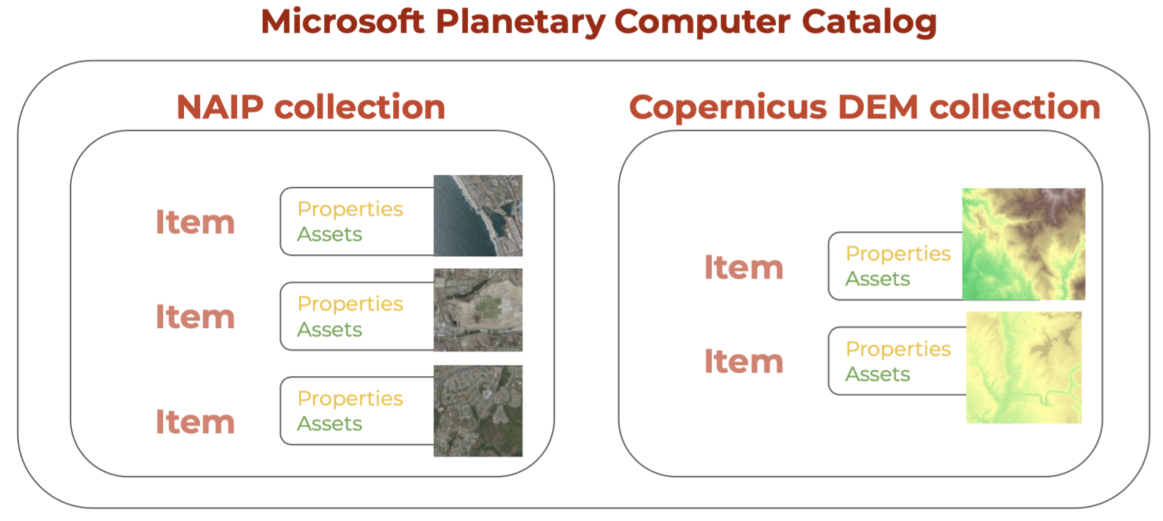
STAC items can be grouped into STAC collections. For example, while a single satellite scene (at a single time and location) would constitue an item, scenes across time and location from the same satellite can be orgnanized in a collection. Finally, multiple collections can be organized into a single STAC catalog.
For example, we’ll be accessing the Microsoft Planetary STAC catalog. Two of its collections are the National Agriculture Imagery Program (NAIP) colelction and the Copernicus Digital Elevation Model (DEM) colleciton. Each of these collections has multiple items, with item cotaining properties (metadata) and assets (links to the data).
25.2 API
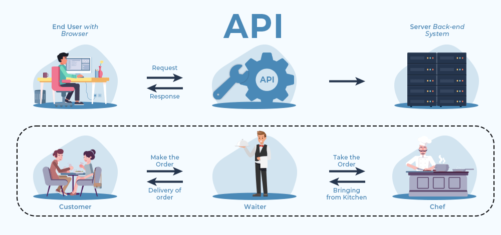
To request data from a catalog following the STAC standard we use an Application Programming Interface (API). We can think of an API as an intermediary tasked with sending our request for data to the data catalog and getting the response from the catalog back to us. The following is a nice real-life analogy:
The Python package to access APIs for STAC catalogs is pystac_client. Our goal in this lesson is to retrieve NAIP data from the MPC’s data catalog via its STAC API.
25.3 Catalog
First, load the necessary packages:
25.3.1 Access
We use the Client function from the pystac_client package to access the catalog:
# access catalog
catalog = Client.open(
    "https://planetarycomputer.microsoft.com/api/stac/v1",
    modifier=planetary_computer.sign_inplace,
)
The modifier parameter is needed to access the data in the MPC catalog.
25.3.2 Exploration
Let’s check out some of the catalog’s metadata:
# metadata from the catalog
print('Title:', catalog.title)
print('Description:', catalog.description)
Title: Microsoft Planetary Computer STAC API
Description: Searchable spatiotemporal metadata describing Earth science datasets hosted by the Microsoft Planetary ComputerWe can access its collections by using the get_collections() method:
catalog.get_collections()<generator object Client.get_collections at 0x112732570>Notice the output of get_collections() is a generator. This is a special kind of lazy object in Python over which you can loop over like a list. Unlike a list, the items in a generator do not exist in memory until you explicitely iterate over them or convert them to a list. Let’s try getting the collections from the catalog again:
# get collections and print their names
collections = list(catalog.get_collections())

print('Number of collections:', len(collections))

print("Collections IDs (first 10):")
for i in range(10):
    print('-', collections[i].id)
Number of collections: 123
Collections IDs (first 10):
- daymet-annual-pr
- daymet-daily-hi
- 3dep-seamless
- 3dep-lidar-dsm
- fia
- sentinel-1-rtc
- gridmet
- daymet-annual-na
- daymet-monthly-na
- daymet-annual-hi25.4 Collection
The NAIP catalog’s id is 'naip'. We can select a single collection for exploration using the get_child() method for the catalog and the collection id as the parameter:
naip_collection = catalog.get_child('naip')
naip_collection- type "Collection"
- id "naip"
- stac_version "1.0.0"
- description "The [National Agriculture Imagery Program](https://www.fsa.usda.gov/programs-and-services/aerial-photography/imagery-programs/naip-imagery/) (NAIP) provides U.S.-wide, high-resolution aerial imagery, with four spectral bands (R, G, B, IR). NAIP is administered by the [Aerial Field Photography Office](https://www.fsa.usda.gov/programs-and-services/aerial-photography/) (AFPO) within the [US Department of Agriculture](https://www.usda.gov/) (USDA). Data are captured at least once every three years for each state. This dataset represents NAIP data from 2010-present, in [cloud-optimized GeoTIFF](https://www.cogeo.org/) format. "
links [] 6 items
0
- rel "items"
- href "https://planetarycomputer.microsoft.com/api/stac/v1/collections/naip/items"
- type "application/geo+json"
1
- rel "root"
- href "https://planetarycomputer.microsoft.com/api/stac/v1/"
- type "application/json"
- title "Microsoft Planetary Computer STAC API"
2
- rel "license"
- href "https://www.fsa.usda.gov/help/policies-and-links/"
- title "Public Domain"
3
- rel "describedby"
- href "https://planetarycomputer.microsoft.com/dataset/naip"
- type "text/html"
- title "Human readable dataset overview and reference"
4
- rel "self"
- href "https://planetarycomputer.microsoft.com/api/stac/v1/collections/naip"
- type "application/json"
5
- rel "parent"
- href "https://planetarycomputer.microsoft.com/api/stac/v1"
- type "application/json"
- title "Microsoft Planetary Computer STAC API"
stac_extensions [] 2 items
- 0 "https://stac-extensions.github.io/item-assets/v1.0.0/schema.json"
- 1 "https://stac-extensions.github.io/table/v1.2.0/schema.json"
item_assets
image
- type "image/tiff; application=geotiff; profile=cloud-optimized"
roles [] 1 items
- 0 "data"
- title "RGBIR COG tile"
eo:bands [] 4 items
0
- name "Red"
- common_name "red"
1
- name "Green"
- common_name "green"
2
- name "Blue"
- common_name "blue"
3
- name "NIR"
- common_name "nir"
- description "near-infrared"
metadata
- type "text/plain"
roles [] 1 items
- 0 "metadata"
- title "FGDC Metdata"
thumbnail
- type "image/jpeg"
roles [] 1 items
- 0 "thumbnail"
- title "Thumbnail"
- msft:region "westeurope"
- msft:container "naip"
- msft:storage_account "naipeuwest"
- msft:short_description "NAIP provides US-wide, high-resolution aerial imagery. This dataset includes NAIP images from 2010 to the present."
- title "NAIP: National Agriculture Imagery Program"
extent
spatial
bbox [] 1 items
0 [] 4 items
- 0 -124.784
- 1 24.744
- 2 -66.951
- 3 49.346
temporal
interval [] 1 items
0 [] 2 items
- 0 "2010-01-01T00:00:00Z"
- 1 "2021-12-31T00:00:00Z"
- license "proprietary"
keywords [] 7 items
- 0 "NAIP"
- 1 "Aerial"
- 2 "Imagery"
- 3 "USDA"
- 4 "AFPO"
- 5 "Agriculture"
- 6 "United States"
providers [] 3 items
0
- name "USDA Farm Service Agency"
roles [] 2 items
- 0 "producer"
- 1 "licensor"
- url "https://www.fsa.usda.gov/programs-and-services/aerial-photography/imagery-programs/naip-imagery/"
1
- name "Esri"
roles [] 1 items
- 0 "processor"
- url "https://www.esri.com/"
2
- name "Microsoft"
roles [] 2 items
- 0 "host"
- 1 "processor"
- url "https://planetarycomputer.microsoft.com"
summaries
gsd [] 2 items
- 0 0.6
- 1 1.0
eo:bands [] 4 items
0
- name "Red"
- common_name "red"
- description "visible red"
1
- name "Green"
- common_name "green"
- description "visible green"
2
- name "Blue"
- common_name "blue"
- description "visible blue"
3
- name "NIR"
- common_name "nir"
- description "near-infrared"
assets
thumbnail
- href "https://ai4edatasetspublicassets.blob.core.windows.net/assets/pc_thumbnails/naip.png"
- type "image/png"
- title "NAIP thumbnail"
roles [] 1 items
- 0 "thumbnail"
geoparquet-items
- href "abfs://items/naip.parquet"
- type "application/x-parquet"
- title "GeoParquet STAC items"
- description "Snapshot of the collection's STAC items exported to GeoParquet format."
msft:partition_info
- is_partitioned True
- partition_frequency "AS"
table:storage_options
- account_name "pcstacitems"
roles [] 1 items
- 0 "stac-items"
25.5 Catalog search
We can narrow down the search within the catalog by specifying a time range, an area of interest, and the collection name. The simplest ways to define the area of interest to look for data in the catalog are:
- a GeoJSON-type dictionary with the coordinates of the bounding box,
- as a list
[xmin, ymin, xmax, ymax]with the coordinate values defining the four corners of the bounding box.
In this lesson we will look for the NAIP scenes over Santa Barbara from 2018 to 2023. We’ll use the GeoJSON method to define the area of interest:
# Temporal range of interest
time_range = "2018-01-01/2023-01-01"

# NCEAS bounding box (as a GeoJSON)
bbox = {
    "type": "Polygon",
    "coordinates":[
        [
            [-119.70608227128903, 34.426300194372274],
            [-119.70608227128903, 34.42041139020533],
            [-119.6967885126002, 34.42041139020533],
            [-119.6967885126002, 34.426300194372274],
            [-119.70608227128903, 34.426300194372274]
        ]
    ],
}

# catalog search
search = catalog.search(
    collections = ['naip'],
    intersects = bbox,
    datetime = time_range)
search
<pystac_client.item_search.ItemSearch at 0x15477bed0>To get the items found in the search (or check if there were any matches in the search) we use the item_collection() method:
items = search.item_collection()
len(items)2This output tells us there were two items in the catalog that matched our search!
items- type "FeatureCollection"
features [] 2 items
0
- type "Feature"
- stac_version "1.0.0"
- id "ca_m_3411935_sw_11_060_20200521"
properties
- gsd 0.6
- datetime "2020-05-21T00:00:00Z"
- naip:year "2020"
proj:bbox [] 4 items
- 0 246930.0
- 1 3806808.0
- 2 253260.0
- 3 3814296.0
- proj:epsg 26911
- naip:state "ca"
proj:shape [] 2 items
- 0 12480
- 1 10550
proj:transform [] 9 items
- 0 0.6
- 1 0.0
- 2 246930.0
- 3 0.0
- 4 -0.6
- 5 3814296.0
- 6 0.0
- 7 0.0
- 8 1.0
geometry
- type "Polygon"
coordinates [] 1 items
0 [] 5 items
0 [] 2 items
- 0 -119.683292
- 1 34.373269
1 [] 2 items
- 0 -119.685448
- 1 34.440724
2 [] 2 items
- 0 -119.754272
- 1 34.439192
3 [] 2 items
- 0 -119.752061
- 1 34.371741
4 [] 2 items
- 0 -119.683292
- 1 34.373269
links [] 5 items
0
- rel "collection"
- href "https://planetarycomputer.microsoft.com/api/stac/v1/collections/naip"
- type "application/json"
1
- rel "parent"
- href "https://planetarycomputer.microsoft.com/api/stac/v1/collections/naip"
- type "application/json"
2
- rel "root"
- href "https://planetarycomputer.microsoft.com/api/stac/v1"
- type "application/json"
- title "Microsoft Planetary Computer STAC API"
3
- rel "self"
- href "https://planetarycomputer.microsoft.com/api/stac/v1/collections/naip/items/ca_m_3411935_sw_11_060_20200521"
- type "application/geo+json"
4
- rel "preview"
- href "https://planetarycomputer.microsoft.com/api/data/v1/item/map?collection=naip&item=ca_m_3411935_sw_11_060_20200521"
- type "text/html"
- title "Map of item"
assets
image
- href "https://naipeuwest.blob.core.windows.net/naip/v002/ca/2020/ca_060cm_2020/34119/m_3411935_sw_11_060_20200521.tif?st=2023-12-07T01%3A22%3A02Z&se=2023-12-08T02%3A07%3A02Z&sp=rl&sv=2021-06-08&sr=c&skoid=c85c15d6-d1ae-42d4-af60-e2ca0f81359b&sktid=72f988bf-86f1-41af-91ab-2d7cd011db47&skt=2023-12-08T01%3A19%3A05Z&ske=2023-12-15T01%3A19%3A05Z&sks=b&skv=2021-06-08&sig=KDgZ9RTP61bQDW47WsfPc/6czFOqQkR7FDSoCZigT8Y%3D"
- type "image/tiff; application=geotiff; profile=cloud-optimized"
- title "RGBIR COG tile"
eo:bands [] 4 items
0
- name "Red"
- common_name "red"
1
- name "Green"
- common_name "green"
2
- name "Blue"
- common_name "blue"
3
- name "NIR"
- common_name "nir"
- description "near-infrared"
roles [] 1 items
- 0 "data"
thumbnail
- href "https://naipeuwest.blob.core.windows.net/naip/v002/ca/2020/ca_060cm_2020/34119/m_3411935_sw_11_060_20200521.200.jpg?st=2023-12-07T01%3A22%3A02Z&se=2023-12-08T02%3A07%3A02Z&sp=rl&sv=2021-06-08&sr=c&skoid=c85c15d6-d1ae-42d4-af60-e2ca0f81359b&sktid=72f988bf-86f1-41af-91ab-2d7cd011db47&skt=2023-12-08T01%3A19%3A05Z&ske=2023-12-15T01%3A19%3A05Z&sks=b&skv=2021-06-08&sig=KDgZ9RTP61bQDW47WsfPc/6czFOqQkR7FDSoCZigT8Y%3D"
- type "image/jpeg"
- title "Thumbnail"
roles [] 1 items
- 0 "thumbnail"
tilejson
- href "https://planetarycomputer.microsoft.com/api/data/v1/item/tilejson.json?collection=naip&item=ca_m_3411935_sw_11_060_20200521&assets=image&asset_bidx=image%7C1%2C2%2C3&format=png"
- type "application/json"
- title "TileJSON with default rendering"
roles [] 1 items
- 0 "tiles"
rendered_preview
- href "https://planetarycomputer.microsoft.com/api/data/v1/item/preview.png?collection=naip&item=ca_m_3411935_sw_11_060_20200521&assets=image&asset_bidx=image%7C1%2C2%2C3&format=png"
- type "image/png"
- title "Rendered preview"
- rel "preview"
roles [] 1 items
- 0 "overview"
bbox [] 4 items
- 0 -119.754272
- 1 34.371741
- 2 -119.683292
- 3 34.440724
stac_extensions [] 2 items
- 0 "https://stac-extensions.github.io/eo/v1.0.0/schema.json"
- 1 "https://stac-extensions.github.io/projection/v1.0.0/schema.json"
- collection "naip"
1
- type "Feature"
- stac_version "1.0.0"
- id "ca_m_3411935_sw_11_060_20180724_20190209"
properties
- gsd 0.6
- datetime "2018-07-24T00:00:00Z"
- naip:year "2018"
proj:bbox [] 4 items
- 0 246978.0
- 1 3806856.0
- 2 253212.0
- 3 3814248.0
- proj:epsg 26911
- naip:state "ca"
proj:shape [] 2 items
- 0 12320
- 1 10390
proj:transform [] 9 items
- 0 0.6
- 1 0.0
- 2 246978.0
- 3 0.0
- 4 -0.6
- 5 3814248.0
- 6 0.0
- 7 0.0
- 8 1.0
geometry
- type "Polygon"
coordinates [] 1 items
0 [] 5 items
0 [] 2 items
- 0 -119.683827
- 1 34.37369
1 [] 2 items
- 0 -119.685956
- 1 34.44028
2 [] 2 items
- 0 -119.753736
- 1 34.438772
3 [] 2 items
- 0 -119.751554
- 1 34.372185
4 [] 2 items
- 0 -119.683827
- 1 34.37369
links [] 5 items
0
- rel "collection"
- href "https://planetarycomputer.microsoft.com/api/stac/v1/collections/naip"
- type "application/json"
1
- rel "parent"
- href "https://planetarycomputer.microsoft.com/api/stac/v1/collections/naip"
- type "application/json"
2
- rel "root"
- href "https://planetarycomputer.microsoft.com/api/stac/v1"
- type "application/json"
- title "Microsoft Planetary Computer STAC API"
3
- rel "self"
- href "https://planetarycomputer.microsoft.com/api/stac/v1/collections/naip/items/ca_m_3411935_sw_11_060_20180724_20190209"
- type "application/geo+json"
4
- rel "preview"
- href "https://planetarycomputer.microsoft.com/api/data/v1/item/map?collection=naip&item=ca_m_3411935_sw_11_060_20180724_20190209"
- type "text/html"
- title "Map of item"
assets
image
- href "https://naipeuwest.blob.core.windows.net/naip/v002/ca/2018/ca_060cm_2018/34119/m_3411935_sw_11_060_20180724_20190209.tif?st=2023-12-07T01%3A22%3A02Z&se=2023-12-08T02%3A07%3A02Z&sp=rl&sv=2021-06-08&sr=c&skoid=c85c15d6-d1ae-42d4-af60-e2ca0f81359b&sktid=72f988bf-86f1-41af-91ab-2d7cd011db47&skt=2023-12-08T01%3A19%3A05Z&ske=2023-12-15T01%3A19%3A05Z&sks=b&skv=2021-06-08&sig=KDgZ9RTP61bQDW47WsfPc/6czFOqQkR7FDSoCZigT8Y%3D"
- type "image/tiff; application=geotiff; profile=cloud-optimized"
- title "RGBIR COG tile"
eo:bands [] 4 items
0
- name "Red"
- common_name "red"
1
- name "Green"
- common_name "green"
2
- name "Blue"
- common_name "blue"
3
- name "NIR"
- common_name "nir"
- description "near-infrared"
roles [] 1 items
- 0 "data"
metadata
- href "https://naipeuwest.blob.core.windows.net/naip/v002/ca/2018/ca_fgdc_2018/34119/m_3411935_sw_11_060_20180724.txt?st=2023-12-07T01%3A22%3A02Z&se=2023-12-08T02%3A07%3A02Z&sp=rl&sv=2021-06-08&sr=c&skoid=c85c15d6-d1ae-42d4-af60-e2ca0f81359b&sktid=72f988bf-86f1-41af-91ab-2d7cd011db47&skt=2023-12-08T01%3A19%3A05Z&ske=2023-12-15T01%3A19%3A05Z&sks=b&skv=2021-06-08&sig=KDgZ9RTP61bQDW47WsfPc/6czFOqQkR7FDSoCZigT8Y%3D"
- type "text/plain"
- title "FGDC Metdata"
roles [] 1 items
- 0 "metadata"
thumbnail
- href "https://naipeuwest.blob.core.windows.net/naip/v002/ca/2018/ca_060cm_2018/34119/m_3411935_sw_11_060_20180724_20190209.200.jpg?st=2023-12-07T01%3A22%3A02Z&se=2023-12-08T02%3A07%3A02Z&sp=rl&sv=2021-06-08&sr=c&skoid=c85c15d6-d1ae-42d4-af60-e2ca0f81359b&sktid=72f988bf-86f1-41af-91ab-2d7cd011db47&skt=2023-12-08T01%3A19%3A05Z&ske=2023-12-15T01%3A19%3A05Z&sks=b&skv=2021-06-08&sig=KDgZ9RTP61bQDW47WsfPc/6czFOqQkR7FDSoCZigT8Y%3D"
- type "image/jpeg"
- title "Thumbnail"
roles [] 1 items
- 0 "thumbnail"
tilejson
- href "https://planetarycomputer.microsoft.com/api/data/v1/item/tilejson.json?collection=naip&item=ca_m_3411935_sw_11_060_20180724_20190209&assets=image&asset_bidx=image%7C1%2C2%2C3&format=png"
- type "application/json"
- title "TileJSON with default rendering"
roles [] 1 items
- 0 "tiles"
rendered_preview
- href "https://planetarycomputer.microsoft.com/api/data/v1/item/preview.png?collection=naip&item=ca_m_3411935_sw_11_060_20180724_20190209&assets=image&asset_bidx=image%7C1%2C2%2C3&format=png"
- type "image/png"
- title "Rendered preview"
- rel "preview"
roles [] 1 items
- 0 "overview"
bbox [] 4 items
- 0 -119.753736
- 1 34.372185
- 2 -119.683827
- 3 34.44028
stac_extensions [] 2 items
- 0 "https://stac-extensions.github.io/eo/v1.0.0/schema.json"
- 1 "https://stac-extensions.github.io/projection/v1.0.0/schema.json"
- collection "naip"
25.6 Item
Let’s get the first item in the search:
# get first item in the catalog search
item = items[0]
type(item)pystac.item.ItemRemember the STAC item is the core object in a STAC catalog. The item does not contain the data itself, but rather metadata and assets that contain links to access the actual data. Some of the metadata:
# print item id and properties
print('id:' , item.id)
item.properties
id: ca_m_3411935_sw_11_060_20200521{'gsd': 0.6,
'datetime': '2020-05-21T00:00:00Z',
'naip:year': '2020',
'proj:bbox': [246930.0, 3806808.0, 253260.0, 3814296.0],
'proj:epsg': 26911,
'naip:state': 'ca',
'proj:shape': [12480, 10550],
'proj:transform': [0.6, 0.0, 246930.0, 0.0, -0.6, 3814296.0, 0.0, 0.0, 1.0]}Just as the item properties, the item assets are given in a dictionary, with each value being a pystac.asset Let’s check the assets in the item:
item.assets{'image': <Asset href=https://naipeuwest.blob.core.windows.net/naip/v002/ca/2020/ca_060cm_2020/34119/m_3411935_sw_11_060_20200521.tif?st=2023-12-07T01%3A22%3A02Z&se=2023-12-08T02%3A07%3A02Z&sp=rl&sv=2021-06-08&sr=c&skoid=c85c15d6-d1ae-42d4-af60-e2ca0f81359b&sktid=72f988bf-86f1-41af-91ab-2d7cd011db47&skt=2023-12-08T01%3A19%3A05Z&ske=2023-12-15T01%3A19%3A05Z&sks=b&skv=2021-06-08&sig=KDgZ9RTP61bQDW47WsfPc/6czFOqQkR7FDSoCZigT8Y%3D>,
'thumbnail': <Asset href=https://naipeuwest.blob.core.windows.net/naip/v002/ca/2020/ca_060cm_2020/34119/m_3411935_sw_11_060_20200521.200.jpg?st=2023-12-07T01%3A22%3A02Z&se=2023-12-08T02%3A07%3A02Z&sp=rl&sv=2021-06-08&sr=c&skoid=c85c15d6-d1ae-42d4-af60-e2ca0f81359b&sktid=72f988bf-86f1-41af-91ab-2d7cd011db47&skt=2023-12-08T01%3A19%3A05Z&ske=2023-12-15T01%3A19%3A05Z&sks=b&skv=2021-06-08&sig=KDgZ9RTP61bQDW47WsfPc/6czFOqQkR7FDSoCZigT8Y%3D>,
'tilejson': <Asset href=https://planetarycomputer.microsoft.com/api/data/v1/item/tilejson.json?collection=naip&item=ca_m_3411935_sw_11_060_20200521&assets=image&asset_bidx=image%7C1%2C2%2C3&format=png>,
'rendered_preview': <Asset href=https://planetarycomputer.microsoft.com/api/data/v1/item/preview.png?collection=naip&item=ca_m_3411935_sw_11_060_20200521&assets=image&asset_bidx=image%7C1%2C2%2C3&format=png>}for key in item.assets.keys():
print(key, '--', item.assets[key].title)image -- RGBIR COG tile
thumbnail -- Thumbnail
tilejson -- TileJSON with default rendering
rendered_preview -- Rendered previewNotice each asset has an href, which is a link to the data. For example, we can use the URL for the 'rendered_preview' asset to plot it:
# plot rendered preview
Image(url=item.assets['rendered_preview'].href, width=500)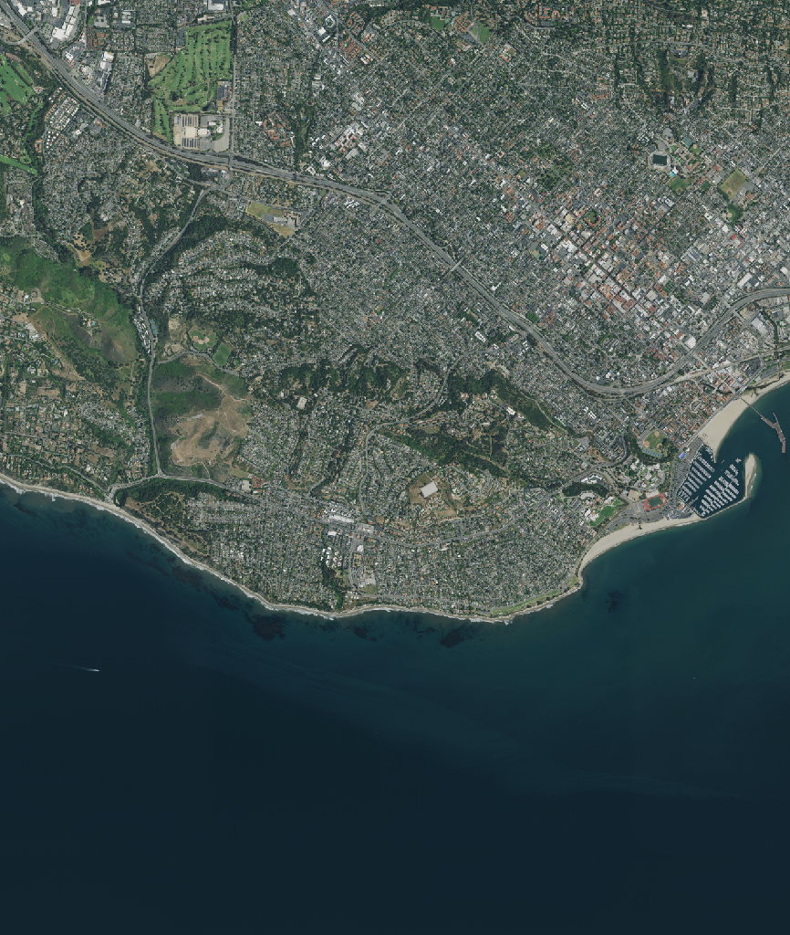
25.7 Load data
The raster data in our current item is in the image asset. Again, we access this data via its URL. This time, we open it using rioxr.open_rasterio() directly:
sb = rioxr.open_rasterio(item.assets['image'].href)
sb
<xarray.DataArray (band: 4, y: 12480, x: 10550)>
[526656000 values with dtype=uint8]
Coordinates:
* band (band) int64 1 2 3 4
* x (x) float64 2.469e+05 2.469e+05 ... 2.533e+05 2.533e+05
* y (y) float64 3.814e+06 3.814e+06 ... 3.807e+06 3.807e+06
spatial_ref int64 0
Attributes:
AREA_OR_POINT: Area
TIFFTAG_IMAGEDESCRIPTION: OrthoVista
TIFFTAG_RESOLUTIONUNIT: 1 (unitless)
TIFFTAG_SOFTWARE: Trimble Germany GmbH
TIFFTAG_XRESOLUTION: 1
TIFFTAG_YRESOLUTION: 1
_FillValue: 0
scale_factor: 1.0
add_offset: 0.0Notice this raster has four bands (red, green, blue, nir), so we cannot use the .plot.imshow() method directly (as this function only works when we have three bands). Thus we need select the bands we want to plot (RGB) before plotting:
# plot raster with correct ratio
size = 6 # height in in of plot height
aspect = sb.rio.width / sb.rio.height
# select R,G,B bands and plot
sb.sel(band=[1,2,3]).plot.imshow(size=size, aspect=aspect)
25.8 Exercise
The 'cop-dem-glo-90' collection contains the Copernicus DEM at 90m resolution data (the data we previously used for the Grand Canyon).
- Reuse the
bboxfor Santa Barbara to look for items in this collection. - Get the first item in the search and check its assets.
- Check the item’s rendered preview asset by clicking on it’s URL.
- Open the item’s data using rioxarray.
25.9 References
STAC Documentation:
Microsoft Planetary Computer Documentation - Reading Data from the STAC API