5  Subsetting

In this lesson we will learn different methods to select data from a pandas.DataFrame.

5.1 Subsetting a pandas.DataFrame

Like it’s often the case when working with pandas, there are many ways in which we can subset a data frame. We will review the core methods to do this.

For all examples we will use simplified data (glacial_loss.csv) from the National Snow and Ice Data Center (Original dataset). The column descriptions are:

• year: ​calendar year
• europe - antarctica: ​change in glacial volume (km3​ ​) in each region that year
• global_glacial_volume_change: ​cumulative​ global glacial volume change (km3), starting in 1961
• annual_sea_level_rise: ​annual rise in sea level (mm)
• cumulative_sea_level_rise:​ cumulative rise in sea level (mm) since 1961

First, we read-in the file and get some baisc information about this data frame:

# import pandas
import pandas as pd

# read in file
df = pd.read_csv('data/lesson-1/glacial_loss.csv')

# see the first five rows
df.head()

	year	europe	arctic	alaska	asia	north_america	south_america	antarctica	global_glacial_volume_change	annual_sea_level_rise	cumulative_sea_level_rise
0	1961	-5.128903	-108.382987	-18.721190	-32.350759	-14.359007	-4.739367	-35.116389	-220.823515	0.610010	0.610010
1	1962	5.576282	-173.252450	-24.324790	-4.675440	-2.161842	-13.694367	-78.222887	-514.269862	0.810625	1.420635
2	1963	-10.123105	-0.423751	-2.047567	-3.027298	-27.535881	3.419633	3.765109	-550.575640	0.100292	1.520927
3	1964	-4.508358	20.070148	0.477800	-18.675385	-2.248286	20.732633	14.853096	-519.589859	-0.085596	1.435331
4	1965	10.629385	43.695389	-0.115332	-18.414602	-19.398765	6.862102	22.793484	-473.112003	-0.128392	1.306939

# get column names
df.columns

Index(['year', 'europe', 'arctic', 'alaska', 'asia', 'north_america',
       'south_america', 'antarctica', 'global_glacial_volume_change',
       'annual_sea_level_rise', 'cumulative_sea_level_rise'],
      dtype='object')

# check the data types of each column
df.dtypes

year                              int64
europe                          float64
arctic                          float64
alaska                          float64
asia                            float64
north_america                   float64
south_america                   float64
antarctica                      float64
global_glacial_volume_change    float64
annual_sea_level_rise           float64
cumulative_sea_level_rise       float64
dtype: object

# data frame's shape: output is a tuple (# rows, # columns)
df.shape

(43, 11)

5.1.1 Selecting a single column…

5.1.1.1 …by column name

This is the simplest case for selecting data. Suppose we are interested in the annual sea level rise. Then we can access that single column in this way:

# seelect a single column by using square brackets []
annual_rise = df['annual_sea_level_rise']

# check the type of the ouput
print(type(annual_rise))

annual_rise.head()

<class 'pandas.core.series.Series'>

0    0.610010
1    0.810625
2    0.100292
3   -0.085596
4   -0.128392
Name: annual_sea_level_rise, dtype: float64

Since we only selected a single column the output is a pandas.Series.

pd.DataFrame = dictionary of columns

Remember we can think of a pandas.DataFrame as a dictionary of its columns? Then we can access a single column using the column name as the key, just like we would do in a dictionary. That is the we just used: df['column_name'].

This is an example of selecting by label, which means we want to select data from our data frame using the names of the columns, not their position.

5.1.1.2 … with attribute syntax

We can also access a single column by using attribute syntax:

annual_rise_2 = df.annual_sea_level_rise
annual_rise_2.head()

0    0.610010
1    0.810625
2    0.100292
3   -0.085596
4   -0.128392
Name: annual_sea_level_rise, dtype: float64

5.1.2 Selecting multiple columns…

5.1.2.1 … using a list of column names

This is another example of selecting by labels. We just need to pass a list with the column names to the square brackets []. For example, say we want to look at the change in glacial volume in Europe and Asia, then we can select those columns like this:

# select columns with names "europe" and "asia"
europe_asia = df[['europe','asia']]

Notice there are double square brackets. This is because we are passing the list of names ['europe','asia'] to the selection brakcets [].

# check the type of the resulting selection
print(type(europe_asia))

# check the shape of the selection
print((europe_asia.shape))

<class 'pandas.core.frame.DataFrame'>
(43, 2)

5.1.2.2 … using a slice

Yet another example of selecting by label! In this case we will use the loc selection. The general syntax is

df.loc[ row-selection , column-selection]

where row-selection and column-selection are the rows and columns we want to subset from the data frame.

Let’s start by a simple example, where we want to select a slice of columns, say the change in glacial volume per year in all regions. This corresponds to all columns between europe and antarctica.

# select all columns between 'arctic' and 'antarctica'
all_regions = df.loc[:,'europe':'antarctica']
all_regions.head()

	europe	arctic	alaska	asia	north_america	south_america	antarctica
0	-5.128903	-108.382987	-18.721190	-32.350759	-14.359007	-4.739367	-35.116389
1	5.576282	-173.252450	-24.324790	-4.675440	-2.161842	-13.694367	-78.222887
2	-10.123105	-0.423751	-2.047567	-3.027298	-27.535881	3.419633	3.765109
3	-4.508358	20.070148	0.477800	-18.675385	-2.248286	20.732633	14.853096
4	10.629385	43.695389	-0.115332	-18.414602	-19.398765	6.862102	22.793484

Notice two things:

• we used the colon : as the row-selection parameter, which means “select all the rows”
• the slice of the data frame we got includes both endpoints of the slice 'arctic':'antarctica'. In other words we get the europe column and the antarctica column. This is different from how slicing works in base Python and NumPy, where the endpoint is not included.

5.1.3 Selecting rows…

Now that we are familiar with some methods for selecting columns, let’s move on to selecting rows.

5.1.3.1 … using a condition

Selecting which rows satisfy a particular condition is, in my experience, the most usual kind of row subsetting. The general syntax for this type of selection is df[condition_on_rows]. For example, suppose we are intersted in all data after 1996. We can select those rows in this way:

# select all rows with year > 1996
after_96 = df[df['year']>1996]
after_96

	year	europe	arctic	alaska	asia	north_america	south_america	antarctica	global_glacial_volume_change	annual_sea_level_rise	cumulative_sea_level_rise
36	1997	-13.724106	-24.832246	-167.229145	-34.406403	-27.680661	-38.213286	-20.179090	-4600.686013	0.909625	12.709077
37	1998	-13.083338	-110.429302	-107.879027	-58.115702	30.169987	-3.797978	-48.129928	-4914.831966	0.867807	13.576884
38	1999	-8.039555	-64.644068	-87.714653	-26.211723	5.888512	-8.038630	-40.653001	-5146.368231	0.639603	14.216487
39	2000	-17.008590	-96.494055	-44.445000	-37.518173	-29.191986	-2.767698	-58.873830	-5435.317175	0.798202	15.014688
40	2001	-8.419109	-145.415483	-55.749505	-35.977022	-0.926134	7.553503	-86.774675	-5764.039931	0.908074	15.922762
41	2002	-3.392361	-48.718943	-87.120000	-36.127226	-27.853498	-13.484593	-30.203960	-6013.225500	0.688358	16.611120
42	2003	-3.392361	-48.718943	-67.253634	-36.021991	-75.066475	-13.223430	-30.203960	-6289.640976	0.763579	17.374699

Let’s break down what is happening here. In this case the condition for our rows is df['year']>1996, this checks which rows have a value greater than 1996 in the year column. Let’s see this explicitely:

# check the type of df['year']>1996
print(type(df['year']>1996))

df['year']>1996

<class 'pandas.core.series.Series'>

0     False
1     False
2     False
3     False
4     False
5     False
6     False
7     False
8     False
9     False
10    False
11    False
12    False
13    False
14    False
15    False
16    False
17    False
18    False
19    False
20    False
21    False
22    False
23    False
24    False
25    False
26    False
27    False
28    False
29    False
30    False
31    False
32    False
33    False
34    False
35    False
36     True
37     True
38     True
39     True
40     True
41     True
42     True
Name: year, dtype: bool

The output is a pandas.Series with boolean values (True or False) indicating which rows satisfy the condition year>1996. When we pass such a series of boolean values to the selection brackets [] we keep only those rows with a True value.

Here’s another example of using a condition. Suppose we want to look at data from years 1970 to 1979. One way of doing this is to use the in operator in our condition:

seventies = df[df['year'].isin(range(1970,1980))]
seventies

	year	europe	arctic	alaska	asia	north_america	south_america	antarctica	global_glacial_volume_change	annual_sea_level_rise	cumulative_sea_level_rise
9	1970	-6.452316	-24.494667	-0.125296	-36.120199	11.619790	11.636911	4.400377	-999.018177	0.110225	2.759719
10	1971	0.414711	-42.904189	28.103328	-8.702938	-9.964542	1.061299	-6.735536	-1038.104459	0.107973	2.867692
11	1972	-5.144729	-27.004031	-22.143350	-40.883357	32.363730	-14.968034	-6.223849	-1122.885506	0.234202	3.101894
12	1973	4.081090	9.839444	22.985188	-31.432594	-20.883232	2.103649	10.539823	-1125.677743	0.007713	3.109607
13	1974	1.545615	-40.126998	-29.517874	-43.861622	-23.991402	-21.338825	4.419343	-1279.964287	0.426206	3.535813
14	1975	7.431192	-32.410467	-44.094084	-43.357442	-30.858810	-2.368842	-7.775315	-1434.818037	0.427773	3.963586
15	1976	3.986753	21.686639	-28.234725	-67.292125	-12.534421	-19.465358	19.250607	-1518.185129	0.230296	4.193882
16	1977	4.891410	-33.123010	-5.662139	-62.165684	-15.905332	2.654950	-23.727249	-1652.453400	0.370907	4.564788
17	1978	8.404591	-77.561015	-12.503384	-22.858040	-31.097609	7.127708	-9.140167	-1791.355022	0.383706	4.948495
18	1979	3.916703	-88.351684	-63.938851	-49.242043	-12.076624	-17.718503	-9.578557	-2030.537848	0.660726	5.609221

Let’s break it down:

• df['year'] is the column with the year values, a pandas.Series,

• in df['year'].isin(), we have that isin is a method for the pandas.Series and we are calling it using the dot ..

• range(1970,1980) constructs consecutive integers from 1970 to 1979 - remember the right endopoint (1980) is not included!

• df['year'].isin(range(1970,1980)) is then a pandas.Series of boolean values indicating which rows have year equal to 1970, …, 1979.

• when we put df['year'].isin(range(1970,1980)) inside the selection brackets [] we obtain the rows of the data frame with year equal to 1970, …, 1979.

loc for row selection

It is equivalent to write

# select rows with year<1965
df[df['year'] < 1965]

and

# select rows with year<1965 using love
df.loc[ df['year'] <1965 , :]

In the second one:

• we are using the df.loc[ row-selection , column-selection] syntax

• the row-selection parameter is the condition df['year']<1965

• the column-selection parameter is a colon :, which indicates we want all columns for the rows we are selecting.

We prefer the first syntax when we are selecting rows and not columns since it is simpler.

5.1.3.2 … using multiple conditions

We can combine multipe conditions by surrounding each one in parenthesis () and using the or operator | and the and operator &.

or example:

# select rows with 
# annual_sea_level_rise<0.5 mm OR annual_sea_level_rise>0.8 mm

df[ (df['annual_sea_level_rise']<0.5) | (df['annual_sea_level_rise']>0.8)]
df.head()

	year	europe	arctic	alaska	asia	north_america	south_america	antarctica	global_glacial_volume_change	annual_sea_level_rise	cumulative_sea_level_rise
0	1961	-5.128903	-108.382987	-18.721190	-32.350759	-14.359007	-4.739367	-35.116389	-220.823515	0.610010	0.610010
1	1962	5.576282	-173.252450	-24.324790	-4.675440	-2.161842	-13.694367	-78.222887	-514.269862	0.810625	1.420635
2	1963	-10.123105	-0.423751	-2.047567	-3.027298	-27.535881	3.419633	3.765109	-550.575640	0.100292	1.520927
3	1964	-4.508358	20.070148	0.477800	-18.675385	-2.248286	20.732633	14.853096	-519.589859	-0.085596	1.435331
4	1965	10.629385	43.695389	-0.115332	-18.414602	-19.398765	6.862102	22.793484	-473.112003	-0.128392	1.306939

and example

# select rows with cumulative_sea_level_rise>10 AND  global_glacial_volume_change<-300
df[ (df['cumulative_sea_level_rise']>10) & (df['global_glacial_volume_change']<-300)]

	year	europe	arctic	alaska	asia	north_america	south_america	antarctica	global_glacial_volume_change	annual_sea_level_rise	cumulative_sea_level_rise
32	1993	16.685013	-73.666274	-43.702040	-65.995130	-33.151246	-20.578403	-20.311577	-3672.582082	0.671126	10.145254
33	1994	0.741751	-3.069084	-59.962273	-59.004710	-89.506142	-15.258449	-8.168498	-3908.977191	0.653025	10.798280
34	1995	-2.139665	-58.167778	-74.141762	3.500155	-0.699374	-19.863392	-25.951496	-4088.082873	0.494767	11.293047
35	1996	-6.809834	-4.550205	-74.847017	-67.436591	4.867530	-21.080115	-11.781489	-4271.401594	0.506405	11.799452
36	1997	-13.724106	-24.832246	-167.229145	-34.406403	-27.680661	-38.213286	-20.179090	-4600.686013	0.909625	12.709077
37	1998	-13.083338	-110.429302	-107.879027	-58.115702	30.169987	-3.797978	-48.129928	-4914.831966	0.867807	13.576884
38	1999	-8.039555	-64.644068	-87.714653	-26.211723	5.888512	-8.038630	-40.653001	-5146.368231	0.639603	14.216487
39	2000	-17.008590	-96.494055	-44.445000	-37.518173	-29.191986	-2.767698	-58.873830	-5435.317175	0.798202	15.014688
40	2001	-8.419109	-145.415483	-55.749505	-35.977022	-0.926134	7.553503	-86.774675	-5764.039931	0.908074	15.922762
41	2002	-3.392361	-48.718943	-87.120000	-36.127226	-27.853498	-13.484593	-30.203960	-6013.225500	0.688358	16.611120
42	2003	-3.392361	-48.718943	-67.253634	-36.021991	-75.066475	-13.223430	-30.203960	-6289.640976	0.763579	17.374699

5.1.3.3 … by position

All the selections we have done so far have been using labels or using a condition. Sometimes we might want to select certain rows depending on their actual position in the data frame. In this case we use iloc selection with the syntax df.iloc[row-indices]. iloc stands for integer-location based indexing. Let’s see some examples:

# select the fifht row = index 4
df.iloc[4]

year                            1965.000000
europe                            10.629385
arctic                            43.695389
alaska                            -0.115332
asia                             -18.414602
north_america                    -19.398765
south_america                      6.862102
antarctica                        22.793484
global_glacial_volume_change    -473.112003
annual_sea_level_rise             -0.128392
cumulative_sea_level_rise          1.306939
Name: 4, dtype: float64

# select rows 23 through 30, inclduing 30
df.iloc[23:31]

	year	europe	arctic	alaska	asia	north_america	south_america	antarctica	global_glacial_volume_change	annual_sea_level_rise	cumulative_sea_level_rise
23	1984	8.581427	-5.755672	-33.466092	-20.528535	-20.734676	-8.267686	-3.261011	-2569.339802	0.232609	7.097624
24	1985	-5.970980	-49.651089	12.065473	-31.571622	-33.833985	10.072906	-13.587886	-2682.857926	0.313586	7.411210
25	1986	-5.680642	22.900847	7.557447	-18.920773	-33.014743	-4.652030	30.482473	-2684.197632	0.003701	7.414911
26	1987	8.191477	12.387780	-24.007862	-41.121970	-48.560996	1.670733	3.130190	-2773.325568	0.246210	7.661120
27	1988	-11.117228	-31.066489	49.897712	-21.300712	-46.545435	13.460422	-37.986834	-2858.767621	0.236028	7.897148
28	1989	14.863220	-23.462392	-36.112726	-46.528372	-57.756422	-21.687470	-10.044757	-3041.169131	0.503872	8.401020
29	1990	-1.226009	-27.484542	-92.713339	-35.553433	-56.563056	-31.077022	-29.893352	-3318.220397	0.765335	9.166355
30	1991	-14.391425	-34.898689	-8.822063	-15.338299	-31.458010	-7.162909	-35.968429	-3467.630284	0.412734	9.579089

Notice since we are back to indexing by position the right endpoint of the slice (6) is not included in the ouput.

5.1.4 Selecting rows and columns simultaneously…

Selecting rows and columns simultaneously can be done using loc (labels or conditions) or iloc (integer position).

5.1.4.1 …by labels or conditions

When we want to select rows and columns simultaneously by labels or conditions we can use loc selection with the syntax

df.loc[ row-selection , column-selection]

specifying both paratmers: row-selection and column-selection. These parameters can be a condition (which generates a boolean array) or a subset of labels from the index or the column names. Let’s see an examples:

# select change in glacial volume in Europe per year after 2000
df.loc[df['year']>2000,['year','europe']]

	year	europe
40	2001	-8.419109
41	2002	-3.392361
42	2003	-3.392361

Let’s break it down:

• we are using the df.loc[ row-selection , column-selection] syntax

• the row-selection parameter is the condition df['year']>1990, which is a boolean array saying which years are greater than 1990

• the column-selection parameter is ['year','europe'] which is a list with the names of the two columns we are intersted in.

5.1.4.2 … by position

When we want to select rows and columns simultaneously by position we use iloc selection with the syntax:

df.iloc[ row-indices , column-indices]

For example,

# select rows 3-7 (including 7) and columns 3 and 4
df.iloc[ 3:8, [3,4] ]

	alaska	asia
3	0.477800	-18.675385
4	-0.115332	-18.414602
5	0.224762	-14.630284
6	-7.174030	-39.013695
7	-0.660556	7.879589

Let’s break it down:

• we are using the df.iloc[ row-indices , column-indices] syntax

• the row-indices parameter is the slice of integer indices 3:8. Remember the right endpoint (8) won’t be included.

• the column-indices parameter is the list of integer indices 3 and 4. This means we are selecting the fourth and fifth column.

5.1.5 Notes about loc and iloc

iloc vs. loc

At the beginning, the difference between iloc and loc can be confusing. Remember the i in iloc stands for integer-location, this reminds us iloc only uses integer indexing to retrieve information from the data frames in the same way as indexing for Python lists.

If you want to dive deeper, this is a great discussion about the difference between iloc and loc: Stackoverflow - How are iloc and loc different?

And, as always, the documentation will provide you with more information: pandas.DataFrame.loc and pandas.DataFrame.iloc.

iloc for column selection? Avoid it!

We can also access columns by position using iloc - but it is best not to if possible.

Suppose we want to access the 10th column in the data frame - then we want to select a column by position. In this case the 10th column is the annual sea level rise data and the 10th position corresponds to the index 9. We can select this column by position using the iloc selection:

# select column by position using iloc
# the syntax is iloc[row-indices, column-indices]
# [:,9] means "select all rows from the 10th column"
annual_rise_3 = df.iloc[:,9]
annual_rise_3.head()

0    0.610010
1    0.810625
2    0.100292
3   -0.085596
4   -0.128392
Name: annual_sea_level_rise, dtype: float64

Unless you are really looking for information about the 10th column, do not access a column by position. This is bound to break in many ways:

• it relies on a person correctly counting the position of a column. Even with a small dataset this can be prone to error.

• it is not explicit: if we want information about sea level rise df.annual_sea_level_rise or df['annual_sea_level_rise'] are explicitely telling us we are accessing that information. df.iloc[:,9] is obscure and uninformative.

• datastets can get updated. Maybe a new column was added before annual_sea_level_rise, this would change the position of the column, which would make any code depending on df.iloc[:,9] invalid. Accessing by label helps reproducibility!

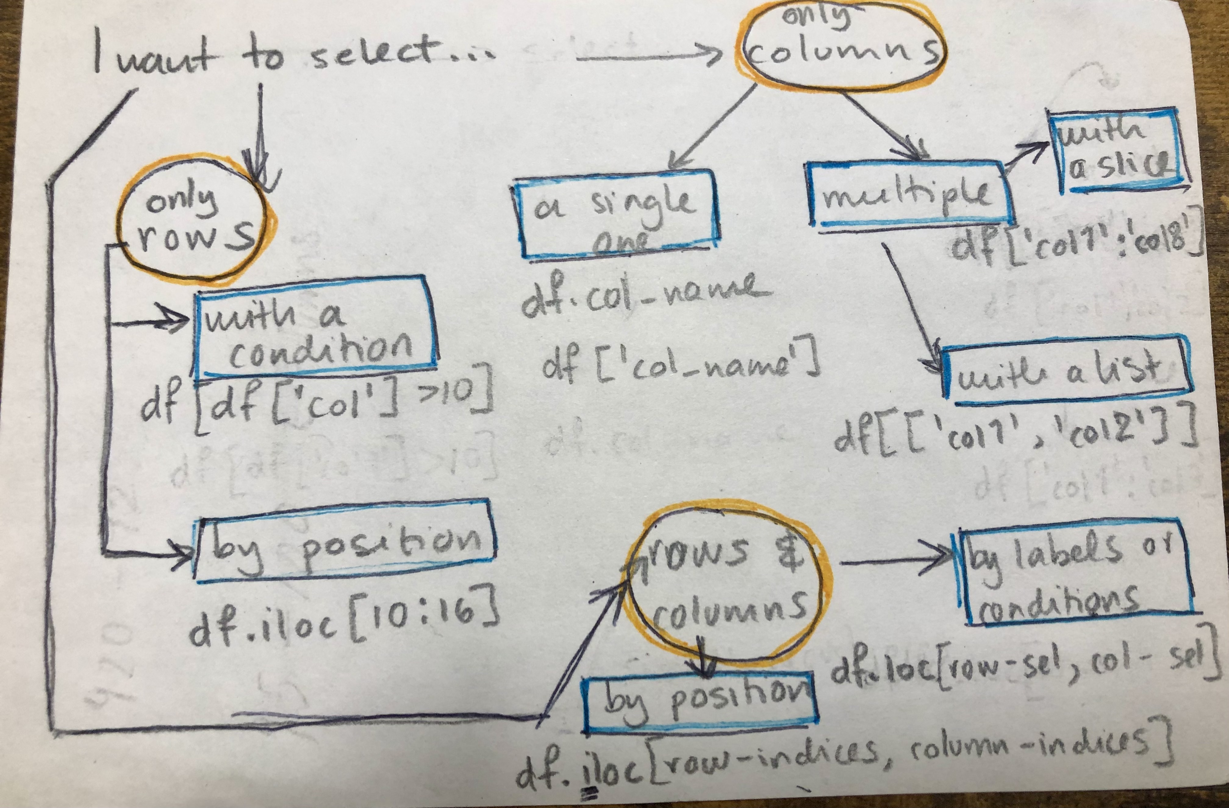
5.2 Summary

pandas.DataFrame selection flow chart

5.3 Resources

What is presented in this section is a comprehensive, but not an exhaustive list of methods to select data in pandas.DataFrames. There are so many ways to subset data to get the same result. Some of the content from this lesson is adapted from the following resources and I encourage you to read them to learn more!

📖 Pandas getting started tutorials - How to I select a subset of a DataFrame

📖 Pandas documentation - User Guide - Indexing and Selecting Data

📖 Python for Data Analysis, 3E - Getting started with pandas

5.4 Acknowledgements

The simplified glacial_loss.csv dataset was created by Dr. Allison Horst as part of her course materials on environmental data science.